More Solar Cycles

July 2, 2024 rjdavison

CSS-58 A recent post by Joseph Fournier highlighted a paper comparing a consolidation of solar cycles to a multi-proxy temperature reconstruction covering the last 1,200 years. The correlation was exceptional. Probably not what the alarmist community wants to see. That correlation does not prove the solar connections, but it does not have to. The only take away you need from this post is the complete lack of influence CO₂ has on the pre-MTR (Modern Temperature Record, 1850 to the present) Holocene temperatures. CO₂ is virtually flat over the pre-MTR Holocene, yet somehow temperatures were still fluctuating significantly?

#climatechange #delaythegreen #globalwarming #showusthedata

The 2017 paper by Lüdecke, H-J., Weiss, C-O., “Harmonic Analysis of Worldwide Temperature Proxies for 2000 Years” analyzed a multi-proxy temperature dataset using a Fourier analysis and found roughly 60-, 190-, 460-, and 1,000-year cycles in the data. The authors used four sinusoidal curves in their evaluation with 60-, 188-, 463-, and 1,003-year frequencies. Can this same analysis be applied to other temperature datasets? This post extends the analysis to Greenland’s GISP2 dataset. Greenland’s very large island status with almost total ice cover and unique position on the planet (intersected by the very important 65 °N Latitude (i.e.: as per Milankovitch’s Insolation Cycle)) amplifies the solar cycle influences. The Lüdecke, Weiss paper uses detrended plots. This analysis leaves the trends in place and extends those trends over the whole Holocene Neoglacial period beginning around 4,000 years ago.

Temperatures are obviously fluctuating significantly throughout the pre-MTR Holocene (in both hemispheres as shown in the attached figure). All with no consequential changes in atmospheric CO₂ concentrations. There are reasons that 65 °N is important in the discussion of deep ice ages, the interglacial warm periods, and the shorter temperature fluctuations throughout. The impacts of solar activity are significantly different over land and ocean. The Northern Hemisphere mid-latitudes (20 to 70 °N) are primarily land and react to solar activity more prominently than the Southern Hemisphere mid-latitude regions (20 to 70 °S). The Milankovitch cycles have correlated very well with global temperatures over the Pleistocene Ice Age.

The same process is still active on shorter time scales. The sun’s energy output (i.e.: Total Solar Irradiance, TSI) remains relatively constant (with a ±0.15% variance). But the insolation (energy input) at 65 °N changes significantly. As an obvious example, we experience seasons yearly. Winter comes every year in the higher latitudes, at annually variable intensity levels. CO₂ is not responsible for those yearly changes; it is the fluctuations in solar insolation. Any parameter (Gamma Ray Flux (cloud cover), high energy particles, electromagnetic field strength, etc.) that affects insolation will affect the climate. That happens on many different time scales. The same processes are active in the Southern Hemisphere (65 °S) with different outcomes due to the ocean’s modulating effects. The Little Ice Age (1300 to 1830) is very prominent in the Northern Hemisphere but is still visible in the Antarctica data.

Based on the GISP data, this evaluation used cycle periods of 60, 190, 460 and 1,150 years. Those durations are open for discussion/adjustment, but they are indicative of natural forcings (most likely solar related). Looking for solar (or solar related) cycle information on the internet turned out to be a frustrating exercise. Generic searches almost invariably returned a site dedicated to the Schwabe cycle, the ±11-year Sunspot cycle. A summary of solar cycles is included below. This list is by no means all inclusive, or definitive. Any additional information on the many cycles would be greatly appreciated.

Cycle Duration Comments

Schwabe ±11-years The Sun Spot Cycle

Hale ±22-years Two Sun Spot Cycles, One full magnetic cycle

AMO-TSI ±60-years The Atlantic Multi-decadal Oscillation, solar related

AMO-Sunshine ±60-years The AMO, sunshine hours, solar related (SR)

ITCZ ±60-years Intertropical Convergence Zone, solar related

SAM Index ±60-years Southern Annular Mode Index, solar related

IAV-Okhotsky Sea ±60-years Interannual Variability, solar related

CCC – Fish Stocks ±60-years Climate Change Cycles and Fish Productivity, SR

THC-Europe ±60-years North Atlantic Thermohaline Circulation, SR

MLA – SSB ±60-years Mid Latitude Aurora and Solar System Barycenter, SR

ISM ±60-years Indian Summer Monsoons, SR

Multi-decadal SSM ±60-years Surface Solar Radiation, SR

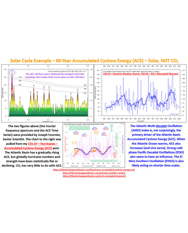
ACE Frequency ±60-years Accumulated Cyclone Energy, Fourier Analysis, SR

ACE Time Series ±60-years Accumulated Cyclone Energy, Time Series, SR

Gleissberg ±88-years

De Vries/Suess ±200-years

GSM ±400-years Grand Solar Minimum frequency

Eddy ±980-years

Bond ±1500-years

Hallstatt ±2400-years

Bray ±2450-years

So, how well does a consolidated four sinusoidal curve fit with the GISP2 data? Definitely not perfect, but a whole lot better than the completely uncorrelated atmospheric CO₂ concentrations. CO₂ concentrations are virtually flat, while temperatures are fluctuating significantly and trending down overall. Over the full Holocene Neoglacial (±4,000 years), the sinusoidal representation highlights all four of the warm periods (Minoan, Roman, Medieval and Modern) and the colder period in between (and to come). The Roman Warm Period is broader in the sinusoidal representation than the GISP data, but still corresponds well overall. The last 900+ years (covering the Medieval Warm Period, the Little Ice Age (LIA), and our Modern Warm Period) correlated extremely well. Much like the Lüdecke, Weiss evaluation. The LIA was the coldest period of the entire Holocene. Not surprising given the overall downward temperature trend and the unrelenting solar minimums (Wolf, Spörer, Maunder, and Dalton) throughout. The sinusoidal representation even accentuated the last Grand Solar Minimum (GSM), the deep cold of the Maunder Minimum (late 1600s).

The same forcings that produced this very real downward temperature trend and the many solar minimum induced cold periods are still active and will continue to lower temperatures in the future. Just not in the All CO₂, All the Time computer model projections. Those same computer models that have been self-acknowledged to “run way too hot” and use unrealistically high emission scenarios. Ignoring the much more important natural forcings (primarily solar through direct and indirect mechanisms) is an extremely dangerous approach. Unfortunately, our ideological “leadership” has opted to embrace that dangerous, financially destructive path. Both sides of the political spectrum are guilty of and promoting their own version of these unnecessary “green” initiatives (Net Zero, ESG, Scope 1, 2, 3 emissions, etc.).

Given the pre-Medieval Warm Period discrepancies (actual temperature fluctuations (while there) were more pronounced than the sinusoidal representation), there may be additional factors to consider. Note, CO₂ is not one of those factors. The answer may be as simple as the Greenland response is just more pronounced than the overall global response has been, and older proxies are not as robust. Regardless, some process is producing rapidly rising temperatures in Greenland, followed by an abrupt switch to rapidly declining temperatures. Again, not CO₂. A possible explanation could be the Dansgaard-Oeschger (DO) events (rapid warming) and subsequent, rapid cooling, Heinrich Events (HE). These events have been recognized numerous times throughout the deep ice age (warming and cooling the planet by ±5 to 15 °C in just decades). Those same processes would still be active throughout the Holocene interglacial warm period, they just appear to be more muted (in the 1 to 2 °C range).

This type of process cannot be displayed as a sinusoidal curve. A better visualization might be a pendulum (a progression of semi-circles with a diameter of 1,150 years). Natural forcings (very likely related to orbital and solar dynamics) are producing an accelerating warming. Those natural forcings obviously reach an infection/tipping (?) point and temperatures abruptly begin falling just as rapidly as they were rising. That process appears to be playing itself out again in our lifetimes. Is CO₂ contributing to the recent temperature rise? Yes, more than likely. But how much? The temperatures started rising before CO₂. The deepest cold of the LIA was in the late 1600s during the Maunder Minimum. Roughly half of the 1.07 °C temperature rise since the pre-industrial area (as per the IPCC’s August 2021 AR6-SPM report) occurred pre-1950. Over 86% of human emissions occurred post-1950. Assuming all the warming post-1950 was due to human emissions (it is not), the warming is beneficial not dangerous.

The overall downward temperature trend is a function of the Milankovitch Cycles, with the Obliquity component being the primary driver over the Holocene. The next step in the evaluation was combining the Pendulum curve with the Obliquity curve. The end result is shown on the last slide. The consolidated Pendulum/Obliquity curve closely matches Greenland’s GISP2 temperature dataset. Is this undeniable scientific evidence that solar activity is responsible for Greenland temperature changes? Absolutely not. But the two consolidations provide possible explanations for the obvious Greenland temperature changes over the Holocene. What is undisputable? There was no CO₂ contribution in the pre-MTR Holocene Greenland temperatures. Greenland temperatures (and by extension global temperatures) have been, are, and will continue to fluctuate with or without CO₂ contribution. A logical next step would be combining the sinusoidal representation with the Pendulum/Obliquity consolidation. An option for another day.

The All CO₂, All the Time narrative is simplistic and unscientific (and in my opinion dangerous). Does this post represent definitive science? No, but the answer definitely does not lie in the alarmist All CO₂, All the Time narrative. For more perspective and more detailed analysis, you can also check out some of the following posts.